Cumulative Distribution Plots for Frequency Data in R

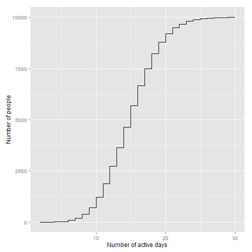
R has some great tools for generating and plotting cumulative distribution functions. However, they are suited for raw data, not when the data is summarized in frequency counts. However, reducing to frequency counts is often necessary when processing data at the scale of tens of gigabytes or more. Here I describe a convenient two-liner in R to plot CDFs in R based on aggregated frequency data.
For example, suppose you want to analyze the number of times people exercise in a month. One option would be to work with a data table consisting of the number of active days for each person.
library(dplyr)
library(ggplot2)
running_log <- data.frame(person_id=1:10000,
                          num_active_days=rpois(10000, lambda=15)) %>%
  transmute(num_active_days=ifelse(num_active_days<=30, num_active_days, 30))
tbl_df(running_log)
## Source: local data frame [10,000 x 1]
##
##    num_active_days
## 1               14
## 2               12
## 3               13
## 4               12
## 5               17
## 6               18
## 7               16
## 8               18
## 9               16
## 10              11
## ..             ...
CDFs from raw data
Using built-in function ecdf, it is easy to generate the cumulative distribution function for such data.
cdf_fun <- ecdf(running_log$num_active_days)
plot(cdf_fun, xlab="Number of active days",
     ylab="Number of people",main="")

For those interested, ggplot provides a function stat_ecdf, which makes this process even simpler.
ggplot(running_log, aes(x=num_active_days)) + stat_ecdf()

CDFs with processed, frequency data
Let us now compress our data by precomputing the frequency of people active on each day.
frequency_counts <- running_log %>% group_by(num_active_days) %>%
  summarize(num_people=n())
frequency_counts
## Source: local data frame [28 x 2]
##
##    num_active_days num_people
## 1                2          1
## 2                4          4
## 3                5         18
## 4                6         55
## 5                7        103
## 6                8        188
## 7                9        328
## 8               10        522
## 9               11        650
## 10              12        847
## ..             ...        ...
Note how this is a 30x2 table at worst, instead of 10,000x2 entries that we started with. Calculating the empirical cumulative distribution involves sorting the data and using cumsum to calculate cumulative sums, then plot using the step function as before.
cumulative_frequencies <- frequency_counts %>%
  arrange(num_active_days) %>%
  mutate(cum_frequency=cumsum(num_people))
cumulative_frequencies
## Source: local data frame [28 x 3]
##
##    num_active_days num_people cum_frequency
## 1                2          1             1
## 2                4          4             5
## 3                5         18            23
## 4                6         55            78
## 5                7        103           181
## 6                8        188           369
## 7                9        328           697
## 8               10        522          1219
## 9               11        650          1869
## 10              12        847          2716
## ..             ...        ...           ...
ggplot(cumulative_frequencies, aes(x=num_active_days, y=cum_frequency)) +
 geom_step() + xlab("Number of active days") + ylab("Number of people")

Bonus: plotting multiple CDFs together
Now, suppose you wanted to break down your analysis by the type of activity. Let us assume that there are two types of activities: running and cycling.
cycling_log <- data.frame(person_id=1:10000,
                          num_active_days=rpois(10000, lambda=15)) %>%
  transmute(num_active_days=ifelse(num_active_days<=30, num_active_days, 30))
activity_log <- rbind(running_log %>% mutate(activity_type="running"),
                      cycling_log %>% mutate(activity_type="cycling"))
frequency_counts = activity_log %>%
  group_by(num_active_days, activity_type) %>%
  summarize(num_people=n())
frequency_counts
## Source: local data frame [56 x 3]
## Groups: num_active_days
##
##    num_active_days activity_type num_people
## 1                2       running          1
## 2                3       cycling          1
## 3                4       cycling          8
## 4                4       running          4
## 5                5       cycling         22
## 6                5       running         18
## 7                6       cycling         60
## 8                6       running         55
## 9                7       cycling        100
## 10               7       running        103
## ..             ...           ...        ...
The same code can be used to generate the CDF, with an additional group_by.
cumulative_frequencies <- frequency_counts %>% group_by(activity_type) %>%
  mutate(cum_frequency=cumsum(num_people))
cumulative_frequencies
## Source: local data frame [56 x 4]
## Groups: activity_type
##
##    num_active_days activity_type num_people cum_frequency
## 1                2       running          1             1
## 2                3       cycling          1             1
## 3                4       cycling          8             9
## 4                4       running          4             5
## 5                5       cycling         22            31
## 6                5       running         18            23
## 7                6       cycling         60            91
## 8                6       running         55            78
## 9                7       cycling        100           191
## 10               7       running        103           181
## ..             ...           ...        ...           ...
ggplot(cumulative_frequencies, aes(x=num_active_days, y=cum_frequency)) +
  geom_step() + facet_wrap(~activity_type) +
  xlab("Number of active days") + ylab("Number of people")
